
The Humboldt-Merger
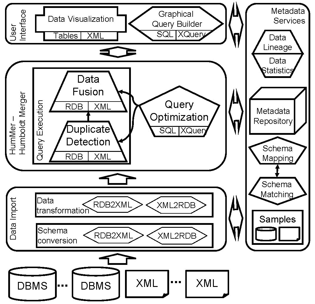

(Picture 1) Architecture of HumMer
The picture shows the architecture of HumMer.


(Picture 2) Data integration process
The Figure shows the steps of the integration process described in Section 2.1
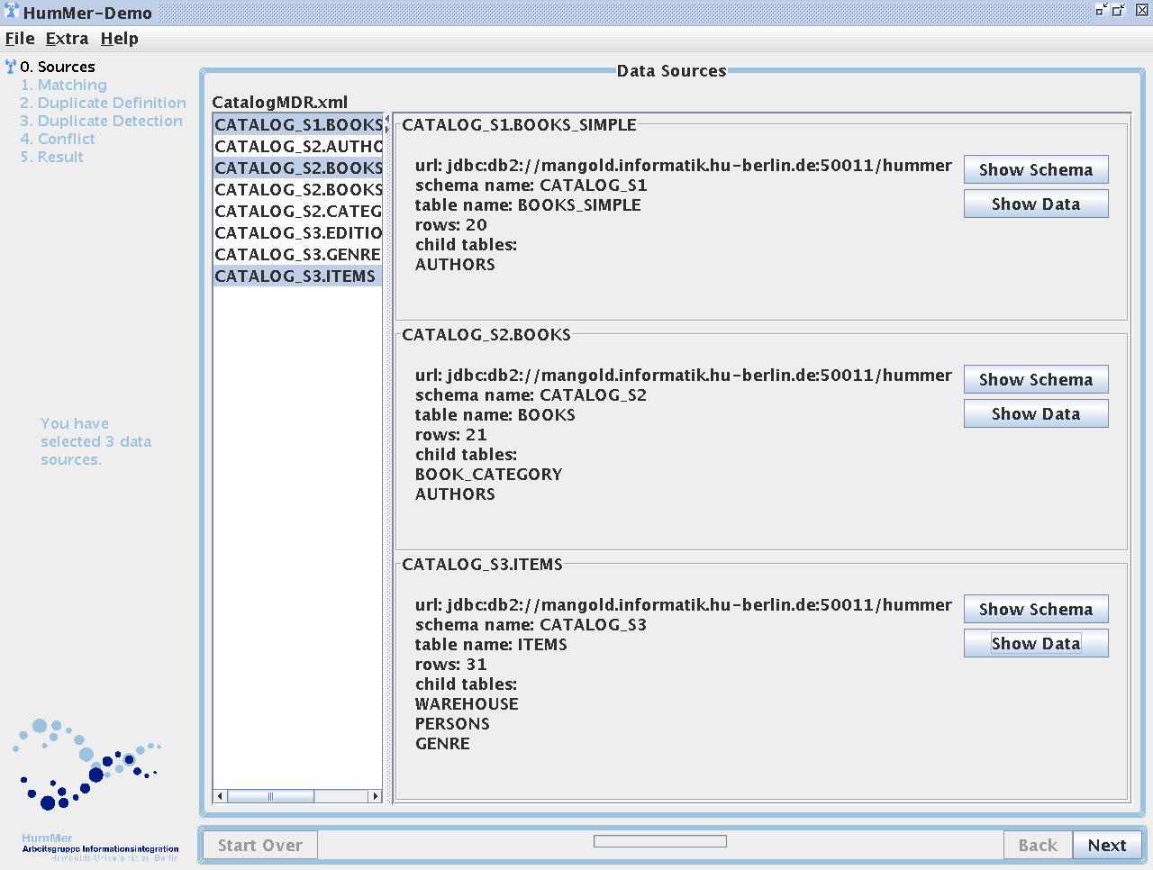
(Screenshot 1) Choosing the data sources
The screenshot shows the visualisation of the first step.
It can be seen that the visualisation consists of two parts.
First the frame and second the visualisation of the step itself (in this case the visualisation supporting the user in choosing data sources).
The frame consits of a navigation bar and buttons to move through the integration process.
The visualisation of the step consists although of two parts: an alias list and informations to the chosen data sources.
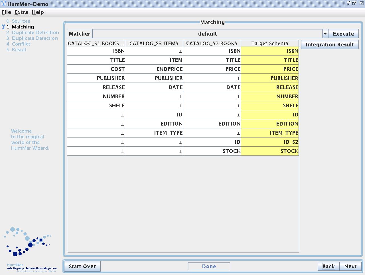
(Screenshot 2) Matching visualisation
The screenshot shows the visualisation of the matching.
The matching is displayed in a table and can be altered by drag and drop functionality.
A button allows to view the integration result based on the matching.
Furthermore, the visualisation of the step contains a combo box at the top to choose the matching algorithm.

(Screenshot 3) Duplicate definition
In this screenshot you can see how duplicates are defined.
The tree structure to the left shows the schema of the integration result.
Below the result schema, the schemas of the child sources of the original chosen data sources are shown.
Selected attributes in the result schema and in the child schemas are used by the duplicate detection step to identify duplicates.

(Screenshot 4) Duplicate detection
This screenshot allows you to take a look at the duplicate detection step.
At this point the automated duplicate detection is already done.
You can see the chosen duplicate detection implementation and the used threshold values at the top.
In the center of the screen a possible duplicate pair is presented to the user with all its attribute values.
Now it is the task of the user to decide whether or not this is a true duplicate based on the values and the calculated similarity of the objects.

(Screenshot 5) Choosing conflict resolution
In this screenshot you can see the integration result presented to the user in a table.
The table data is segmented into groups. These groups are marked by alternating colours.
Each group represents the same real world object.
The table header allows the user to choose a conflict resolution function for each attribute column of the integration result.

(Screenshot 6) Conflict resolution functions
Here you can see the visualisation the user can choose a conflict resolution from.
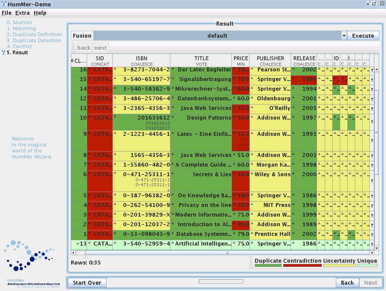
(Screenshot 7) Result
The result is visualised in a table with coloured table cells.
The colour of each cell indicates the relations between the values of the duplicates fused to the value in the cell.
A icon inside the cell enables the user to examine these duplicate values and check the result of the conflict resolution function.
Another icon at the end of each row allows the user to examine the provenance of the result tuple.
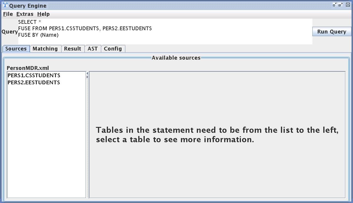
(Screenshot 8) SQL GUI
The screenshot shows the SQL GUI of HumMer.
At the top of the image you can see a simple example of a FUSE BY statement.
Below the query is a list and descriptions of the available data sources.
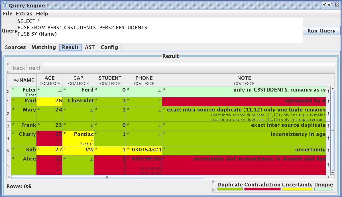
(Screenshot 9) SQL GUI result
Here you can see the result of a FUSE BY statement.
The visualisation of the result is exactly the same as introduced in Section Step 6.
1) What is HumMer?
The Humboldt-Merger (in short: HumMer) is a part of the Merging Autonomous Content project at the Humboldt-Universität zu Berlin.
HumMer is an integrated information system, reading relational, XML, and unstructured data and merging it into common, structured information.
HumMer proceeds in three steps:
First, schema matching bridges schematic heterogeneity of the data sources by aligning corresponding attributes.
Next, duplicate detection techniques find multiple representations of identical real-world objects.
Finally, data fusion and conflict resolution merges duplicates into a single, consistent, and clean representation.
1.1) Project members
-
Prof. Felix Naumann (Project director)
-
Melanie Weis (Duplicate detection)
-
Jens Bleiholder (Data fusion)
-
Christoph Böhm (XQuery generator and GUI)
-
Karsten Draba (GUI and HumMer framework development)
-
Alexander Bilke (Schema matching)
1.2) Related work
- [BilkeBBDNW05]A. Bilke, J. Bleiholder, C. Böhm, K. Draba, F. Naumann and M. Weis. Automatic Data Fusion with HumMer. In Proceedings of the 31st International Conference on Very Large Data Bases, Trondheim, Norway, August 30 - September 2, 2005, pages 1251-1254, 2005
- [BilkeN05]A. Bilke. Schema matching using Duplicates. In Proceedings of the 21st International Conference on Data Engineering, ICDE 2005, 5-8 April 2005, Tokyo, Japan, pages 69-80, 2005
- [BleiholderN05]J. Bleiholder. Declarative Data Fusion - Syntax, Semantics, and Implementation. In Advances in Databases and Information Systems, 9th East European Conference, ADBIS 2005, Tallinn, Estonia, September 12-15, 2005, Proceedings, pages 58-73, 2005
- [Draba05]K. Draba. Visualisierung fusionierter relationaler Daten (Studienarbeit)., April 2005
- [WeisN05]M. Weis. DogmatiX Tracks down Duplicates in XML. In Proceedings of the ACM International Conference on Management of Data (SIGMOD) 2005, Baltimore, Maryland, USA, 2005
1.3) A framework and system for data integration
The aim of HumMer is to provide researchers with an easy way of implementing and testing new ideas concerning the information integration process. It serves as a plattform to test the feasability, scalability, and usefulness of new ideas.
Therefore, a framework is needed allowing researchers not only to implement new parts of an integration process but also supporting them to install the implementation into the integration process itself.
Whether a new solution for an old task is to be tested or a completely new task is to be installed in the integration process, HumMer provides a means to do so.
While still under development, a first demonstration, called "Automatic Data Fusion with HumMer" [BilkeBBDNW05], was given to the interested public at the VLDB 2005.
Picture 1 provides an overview of HumMer architecture.
1.4) Integration as a series of steps
In the world of HumMer a data integration task is regarded as a series of data integration steps.
HumMer allows researchers to build such series by creating XML configuration files.
In other words HumMer allows the researcher a step by step integration control of all important integration steps.
In general, each step visualises the output of the previous step and provides the input for the next one.
Default values enable the researcher to ignore all steps he/she is not interested in and enable to proceed to the next step without taking care of the current one.
To test new algorithms a step can be repeated, new algorithms can be chosen and new parameters can be set.
And of course the entire process can be restarted at any time.
Although the aim of HumMer is to provide a tool that is able to integrate data from different kind of data sources (e.g. relational data, XML data, and delimited text data), the visualisation is based on the relational model and often represents the data in tables to the user.
Therefore, while talking about rows and columns in the visualisation we do not restrict HumMer to relational data.
2) What does HumMer look like?
This section describes the graphical user interface (GUI) of HumMer. HumMer has two different GUI's.
First the wizard GUI is described and second the SQL GUI.
2.1) The Wizard or How to drive a HumMer by yourself?
The Wizard is driven by user interaction and visualises the steps of the integration process.
The visualisation can be divided into two parts:
First a frame that is the same for all integration steps and second the visualisation of each step.
In the following an integration process is assumed to consist of six steps. (shown in Picture 2)
-
Choose data sources
-
Match attributes and integrate the chosen data sources
-
Identify attributes that define objects
-
Detect duplicate objects
-
Choose a conflict resolution and fuse objects
-
Check the integrated result
2.1.1) The frame of the Wizard
As can be seen in Screenshot 1 the frame holds all the steps together.
It helps orientation and moving through the integration process.
Forward and backward navigation are possible. It is also possible to restart the entire process.
A navigation bar shows the current step as well as the steps already passed and the steps to come.
A simple status bar shows the progress of the current step.
A small message area allows to display information helping the user to proceed.
Most of the space is reserved for the representation of each individual step.
This space is also used to display information to the user when proceeding to the next step.
2.1.2) Visualisation of steps in general
Before going into the details of visualisation of each step proposed in Section 2.1 a few general things about the representation of a step may be considered.
Regard Screenshot 2.
In general each step visualises the result of the step before and delivers the input to the next step.
Whatever is done in the current step can influence the following steps.
A step is destined to fulfil a certain task. In most cases how this task is to be acomplished depends on the algorithm implementing the task.
Hence many implementations can fulfil a certain task and an easy way to choose a certain implementation is essential for the user to test implementations and compare them with each other.
Therefore the visualisation of a integration step provides a pull down menu to choose the implementation to use.
In some steps additional parameters of the algorithm can be set.
But most steps do not require any input at all; using the default values will just do fine in most cases.
2.1.3) An example for the visualisation of an integration process
In the following paragraphs we will give an example of the integration process realized in the HumMer demo system.
Each paragraph gives a brief description of the GUI of a step, providing an insight into the possibilities of the user to examine, evaluate and alter the integration process.
Step 1) Choosing the data sources
In Screenshot 1 you can see the visualisation of the first integration step.
The first step allows the user to choose the data sources to integrate.
All available data sources are represented by an alias shown on the left side of the screen.
To register a data source with the hummer, a meta data repository is used.
The meta data repository GUI is introduced in Section 2.3.
To all data sources chosen in the list additional informations are displayed, such as the size of the data source and the name of the child data, which becomes important for duplicate detection (Section Step 3 and Section Step 4).
The user can also take a look at the data and the schema of the selected sources.
Step 2) Schema matching and the integration of the data sources
The second step involves the matching and the integration of the data sources. The visualisation of the step is shown in Screenshot 2.
In fact matching and integration are two different steps, but from the users point of view they can be regarded as one, because the user only takes influence in the integration result by altering the matching.
Furthermore, the integration result is an important indicator for the correctness of the matching and therefore examining both at the same time can be beneficial.
By entering the second step the default matcher implementation is used and the result is shown to the user.
If the result is not satisfactory, the matching can either be altered or another implementation can be used.
A possible matching algorithm used by HumMer is the Dumas approach.
For a short description of Dumas take a look at [BilkeBBDNW05] or go into detail with [BilkeN05].
The matching is displayed in a table, where each column represents the schema of one of the selected data sources and the last column represents the integrated target schema.
A row of the matching table represents a matching between all columns of the selected data sources in it.
The name in the last column of a row is the target column name of the matching.
There are two ways of altering the matching. One is to change the matching itself by dragging the name of a data source column and dropping it at another position in the same column.
If the column is dropped at an empty cell it is matched with all the other source columns in the same row.
And if the column is dropped at a non empty cell or itself a new row is created and therefore a new column in the result schema.
The other way to alter the matching is by editing the names of the result columns in the last column of the table.
The integration result can help to validate the chosen matching, by visualising the integrated data based on the matching and therefore providing the possibility of instance based validation.
Whenever the user wants to see the integration result based on her matching she can start integration by using the appropriate button on the right.
Step 3) The definition of a duplicate
After integrating all the heterogenous data sources it is time to detect duplicates in the result.
Before starting duplicate detection it is necessary to define the attributes that identify a real world object and therefore are to be used for duplicate detection.
Regard Screenshot 3.
There, one can see how duplicates are to be defined.
At the left of the visualisation is a tree structure.
The first node and it child nodes represent the schema of the integration result as created in the previous step.
Each node below the result schema represents the schema of a child source of the original chosen data sources (what is meant by a child source is explained above in Section Step 1).
The comment in the last column gives the user a hint where the information comes from.
In the integration result schema the comment tells the user which source columns where matched to the current one.
I.e., the comment reflects the previously defined matching (as described in Section Step 2).
Further, the comments in the child tables give the user a clue about the child table's origin and how child tables are matched with each other.
This GUI is derived from the GUI of the XQuery Generator.
The duplicate definiton generator which can be chosen through the combo box at the top is used to build the description of the objects used in the next step.
Step 4) The duplicate detection
After duplicate definition, the detection of duplicates is the next step.
Again it is possible to choose different implementations.
The default algorithm is the Dogmatix algorithm introduced in [WeisN05].
A shorter description of this algorithm is also provided in [BilkeBBDNW05].
To render the duplicate detection as effective as possible, a few threshold parameters can be provided to the algorithm.
Based on the specified threshold values the duplicate detection algorithm assigns object pairs to three different classes.
These are non duplicates, sure duplicates, and possible duplicates.
Only possible duplicates are presented to the user as shown in Screenshot 4.
Now it is up to the user to decide for each possible duplicate pair whether or not it is a duplicate.
All duplicate pairs the user has not classified manually are regarded as true duplicates.
As one can see in Screenshot 4, a duplicate pair is visualised as a table.
The first column contains the attribute name, the second the values of the first object and the last the values of the other object.
An easy comparison is made possible by highlighting conflicting values with a different colour from equal values.
The calculated similarity measure is displayed above the table and some statistics like the number of sure duplicates and the number of possible duplicates ahead are shown at the right side.
Step 5) Conflict resolution
In the previous step duplicates where identified and duplicate cluster built.
All objects in a cluster represent the same real world object.
The Screenshot 5 shows the visualisation of these clusters.
Clusters are recognized by their cluster-id in the first column and by a colour alternating from cluster to cluster.
In addition to the cluster-id another column is added to the result schema - the data source column.
This column contains the lineage of the object and tells the user where the data in a row comes from.
Now that we know the duplicates, the next step is to fuse them together to a single consistent representation of their real world object.
To do so a conflict resolution must be chosen.
The idea of conflict resolution functions in HumMer project is based on the FUSE BY statement introduced in [BleiholderN05].
Again a short introduction can be found in [BilkeBBDNW05].
The user can choose a conflict resolution function for each data column by using the button in the header of the table.
This function is applied by group on all conflicts in the column.
Screenshot 6 shows you some of the conflict resolution functions the user can choose from.
Step 6) The result of the integration process
Finally the data fusion is complete and it is time to explore the result of the process.
The result is again presented in a coloured table to the user, as can be seen in Screenshot 7.
And like in Section Step 4 the colour is a hint to conflicts.
Now all duplicates in a cluster (see Section Step 5) are fused together and each row in the table is the representation of a different real world object.
The final step allows the user to check the results and to investigate the consequences of the previous choices.
HumMer supports the user in doing so by helping find interesting values and helping understand their lineage.
Finding interesting values is made easier by highlighting conflicts, uncertainties, duplicates, and unique values.
In addition the rows are sorted by the count of their conflicts.
If interesting values have been found their lineage can be explored by expanding a cell and making the fused values and their origin visible.
Also the lineage of the entire row can be explored by using the icon in the last column.
A more detailed description of the GUI is given in [Draba05].
2.2) The SQL Gui or How to drive a HumMer by query?
The SQL GUI is an alternative to the Wizard introduced above.
Strictly speaking, the SQL GUI provides an implementation of the FUSE BY statement introduced in [BleiholderN05].
In contrast to the Wizard the SQL GUI does not reflect the step by step aspect of the integration process.
Instead of asking the users to make decisions during the process, all decisions are gleaned from the FUSE BY statement.
Screenshot 8 shows an example of a FUSE BY statement and Screenshot 9 a result.
2.3) The meta data repository
Before users can integrate data sources they must register these data sources to HumMer.
The meta data repository GUI provides an easy way to do this.
Only registered data sources are available in the alias list of the first step.
The meta data repository GUI supports the user in creating, loading and storing meta data about data sources.
The meta data itself is stored in a XML file.