Hasso-Plattner-Institut
Prof. Dr. Tilmann Rabl
 

Developing a Benchmark for Real-Time Analytics Systems

written by Tarik Alnawa, Fabian Georgi, Jan Reppien, Gerd Rössler and Finn Schoellkopf

Driven by the increasing volume and velocity of data, stream processing systems have become more and more relevant, not only for tech companies but also for businesses in logistics, finance, and other sectors. Similarly, time-critical business decisions benefit from real-time data analytics. Modern hardware lays the technical foundation for such analytics. Entry hurdles for end users are lowered through cloud computing and analytical systems such as Spark Streaming and Flink. Today, it is easier than ever before to capitalize on real-time analytics.

What is Real-Time Analytics?

Real-time analytics involves using data as soon as it is produced to reason business decisions. Systems need to execute analytical queries, incorporating fresh data. Two metrics are particularly important in this context: - Data Latency: Data latency measures the time it takes for generated data to become visible in a query. For real-time analytics systems, the goal is to minimize this time span during which the data is processed by the systems. Therefore, data should be visible within a few seconds or even sub-seconds. - Query Latency: Query latency is the time it takes for queries to execute and return the result set. Although there are options for quickly inserting data, in the past this has resulted in long query latency. The goal of real-time analytics systems is to minimize query latency and quickly reflect changes in the data. This enables faster business decisions, real-time predictions, and process automation.

The Current State of Benchmarks

Despite the availability of benchmarks such as TPC-H and StarSchema Benchmark (SSB) to assess OLAP system performance, none of these benchmarks adequately address the unique challenges posed by real-time analytics, such as data freshness and streaming ingest capabilities. At the opposite end of the spectrum lie streaming benchmarks, which focus on assessing the performance of stream processing engines but overlook the critical aspect of analytical queries. Examples of such benchmarks include the LinearRoad Benchmark and the Yahoo Streaming Benchmark. To our knowledge, there is no benchmark that combines these two aspects and measures performance of stream processing engines for relational mixed OLTP-OLAP workloads.

Our Goal

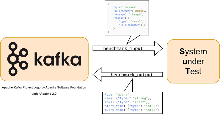
In our master project, we aimed to develop a benchmark specifically designed for realtime analytics systems. The benchmark focuses on data latency and query latency. Our goal was to combine the advantages of streaming systems with a persistent data store, where we can later execute OLAP queries on both the streamed data and the static data. The benchmark must be designed to allow developers of real-time analytics systems to easily test their implementations of different systems, or to find the most efficient implementation for one specific system.

Database Schema

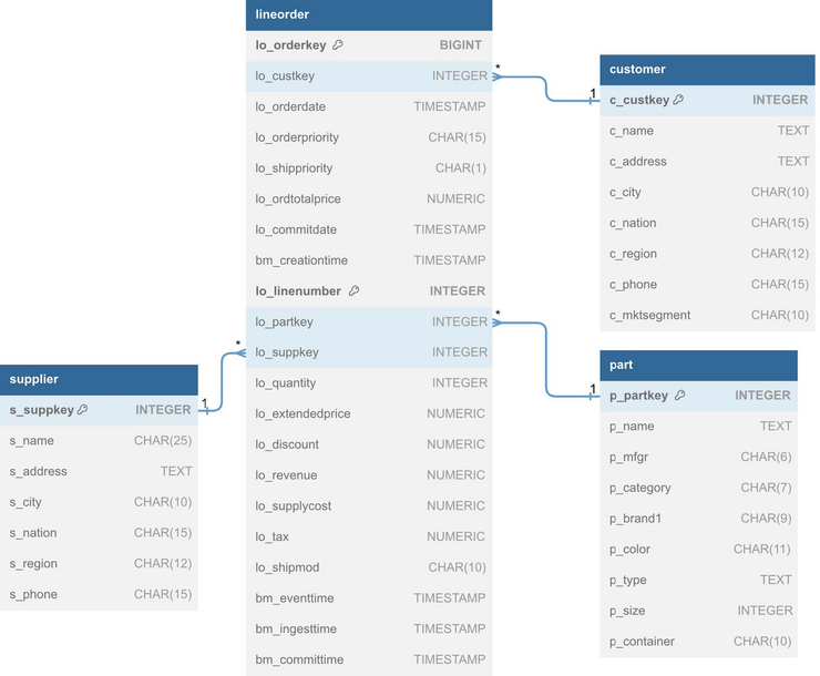
We used the database schema from the StarSchema Benchmark (SSB) as a starting point. The schema includes the customer, part, supplier, and lineorder relations. The latter is a denormalized form of the lineitem and orders table of the well known TPC-H benchmark. Compared to the SSB, we removed the date table and added individual columns for different timestamps, which are labeled with the prefix bm_. Those are used
to track the time spent in the system by each record.

The schema can be seen in the figure below.

Architecture

The benchmark itself consists of four main components

1. Data Generator
2. Message Broker
3. System under Test (SUT)
4. Evaluation

The following graphic provides an overview of our architecture. Below, we will explain each of these components to provide a better understanding of them.
 

Data & Event Generation with EEVEE

Our data generator is called EEVEE and is the result of a master’s thesis at HPI. With EEVEE you can define table schemas which are then used to generate the data. The data is generated deterministically, which is necessary for comparable benchmark runs. Using template specializations, which are instantiated at compile time, EEVEE can generate the data extremely quickly at runtime. Even in single-threaded operation, it can achieve a data throughput of up to 1 GB/s. In addition, state machines are used to track semantic dependencies in the generated data. In our case, EEVEE generates data for new line orders. Using so-called stateful streams, which work internally with state machines, it also sends update or delete instructions for individual line orders.

These three distinct events manifest as follows: 1. create: This event includes new entries for lineorder stored in a nested JSON format. All entries share the same orderkey and belong to a single order. Since each order can contain items, systems must flatten these JSONs structures to generate insertion statements for each item. 2. update: This event removes a single item from the order or modifies the quantity of an existing item within the order. 3. cancel: This event cancels the whole order.

State machine with probabilities of the events.

Additionally EEVEE periodically sends OLAP-Queries, the system has to execute and return the results.

Queries

Our current implementation provides six different queries with different compute loads and result set sizes to represent a range of potential OLAP query use cases. The intervals of each query can be adjusted as needed. Currently, all six queries are sent every 100 1.. n events.

The six implemented queries are: 1. Return all ordered parts along with the number of orders for each part. 2. Return the average discount per category of parts for each supplier. 3. Return the average order price for each customer. 4. For each city, return the minimum, maximum, and average delivery time (the difference between the commit date and the order date). 5. Return the amount of orders per order priority for each nation. 6. Return the maximum delivery time for orders where the supplier and customer are located in the same city, region, and nation, in descending order for each city.

All six queries are templated and include only the data from the last minutes. The size of this timespan can be defined in EEVEE.

Queries can be written in any query language, allowing the benchmark to run with any system. One of our System under Test, DuckDB, required a slightly different SQL syntax.
This was easily achieved by creating a new configuration file for the data generator.

This flexible approach using a configuration file for queries enables users to add their own queries, if they want to use the benchmark to compare systems with queries close to their workloads.

Message Broker

To standardize an interface, we use Apache Kafka as a message broker. The advantage of using a message broker is that a queue is created in which data generation and processing can take place independently of each other. This allows EEVEE to consistently generate data without having to wait for the system under test to acknowledge the message. As a result, we can measure the waiting time in the queue, which provides information about the ingest throughput that the system under test can achieve. We use two different topics in our Apache Kafka setup: benchmark_input and benchmark_output. As the names suggest, the input topic contains all data coming from EEVEE (inserts, updates, deletes, and query events). When the system under test executes these OLAP queries, the result size and the execution time of the query are sent to the output topic, where our evaluation system can retrieve the data.

Systems under Test

Although the main goal of this project was to create a framework and a sample specification, we needed practical implementations to evaluate our efforts. We developed three different implementation examples: - Apache Spark and Postgres - Apache Flink and Postgres - DuckDB

The first two combinations utilize widely adopted systems for stream processing along with Postgres for persistent storage, whereas DuckDB is an in-process database tailored for OLAP queries. We chose these three systems to compare Spark and Flink, and to showcase the benchmark’s versatility with DuckDB by directly integrating persistent storage without requiring an intermediary data processing framework.

Evaluation

As a tuple passes through the various components of the benchmark, it generates three timestamps (see: Architecture-Graphic):

  • bm_eventtime: the time it gets written into Kafka queue

  • bm_ingesttime: the time it is ingested into the System under Test

  • bm_committime: the time it is persisted into the database and therefore query-able

All of these timestamps are persisted in the database, providing valuable information on how long each tuple spent in each component. After the benchmark, we extract all rows with these three timestamps from the database and create a CSV dump. For every tuple we calculate two metrics based on the collected timestamps: - Time in

Queue = bm_ingesttime - bm_eventtime - Processing Time = bm_committime -
bm_ingesttime

For queries, we measure the execution time of the query and the size of the result set (to verify that there is no empty result and thus no error in the system or in the query itself). When the benchmark is finished, we calculate metrics, plot graphs, and save the csv dumps for further analysis as desired. Before we go into the results, let’s take a look at the configurations with which the benchmark was run for the individual systems.

Benchmark Configuration

The following configuration was used for Flink and Spark to achieve the results shown in
the next sections: - EEVEE: - 8 Cores - 16 GB memory - Zookeeper/Kafka (1x
Zookeeper node, 2x Kafka nodes): - Replication Factor: 2 - Partitions: 3 - 32 Cores - 64
GB memory - Postgres: (config created using PGTune) - 256 Cores - 256 GB memory -
Flink (1x master, 1x worker): - 20 Cores - 256 GB memory - Window size: 1000ms -
Spark (1x master, 1x worker): - 20 Cores - 256 GB memory - Window size: 1000ms

Spark

1500 Events per second

Tuples per second: 4500.6841 Avg Time In Queue Per Tuple: 544.2292ms Avg Processing Time Per Tuple: 0.3538s

2500 Events per second

Tuples per second: 7501.4321
Avg Time In Queue Per Tuple: 539.6465ms
Avg Processing Time Per Tuple: 0.3664s

These two diagrams show that Spark can handle the chosen benchmark load without any backpressure. Each event generated by EEVEE spends approximately 500ms in the Kafka queue. This is the expected value for a batch interval time of 1000ms. The processing time for both benchmark runs, from ingest in Spark to being written to Postgres, is around 0.36s. Spark achieves a throughput of 7.5k tuples written to Postgres per second.

Both graphs show occasional spikes in processing time and Kafka queue time, which are likelycaused by the Java garbage collector pausing all threads. If we look at a query (Q1), we can see that the query time increases more or less linearly.
The number of rows in the result set becomes constant after a while, because about as many tuples fall out of the window as new ones come in.

Flink

300 Events per second

Tuples per second: 536.4021 Avg Time In Queue Per Tuple: 30584.0408ms Avg Processing Time Per Tuple: 17.0663s

We found that with the current implementation of the Flink application, even with a small number of events per second, Flink runs into backpressure, causing the average time a tuple spends in the Kafka queue to increase rapidly. The observations show that most of the time is spent writing to the Postgres database using the Flink JdbcSink. It is very unlikely that the Postgres database is the bottleneck in this scenario, as Spark and also Pgbench show that higher throughput is possible with the same database configuration. Due to the nearing end of this project, we were unable to do any further investigation. A possible reason for this problem could be related to the inner workings of JdbcSink or simply a wrong configuration or implementation on our site. Although both Spark and Flink use the same systems (except for the System under Test) and configurations, our benchmark shows significant performance differences between the two systems that are easily identifiable through visualization and quantitative metrics.

DuckDB

Due to time constraints, we were only able to run DuckDB on a local, single-node setup with 8 cores and 16GB of memory for the entire benchmark (shared with EEVEE, Zookeeper/Kafka, and the evaluation system). We chose a window size of 1000ms.

200 Events per second


Tuples per second: 239.6161
Avg Time In Queue Per Tuple: 187300.8556ms
Avg Processing Time Per Tuple: 2.1832s

Our current implementation for DuckDB supports all of our benchmark metrics, but can’t handle a high number of events per second. Almost immediately, the system runs into backpressure, similar to our implementation with Flink. The average queue time for a tuple increases linearly over the entire run.

Since the DuckDB implementation was meant to show the flexibility of our benchmark to adapt to different types of systems, we didn’t spend the extra time to improve DuckDB’s
performance.

The purpose of a benchmark is to show differences between systems and provide a basis for comparison between them. In this sense, we can say that our benchmark fulfills this purpose by showing performance differences between different systems and different implementations through objective metrics and visualizations. This helps users choose the best system for their needs or compare their implementation with others.

Conclusion & Known Limitations

In summary, our benchmark effectively identifies performance differences between different real-time analytics systems. We have developed a highly customizable benchmarking framework that is easily configurable for different use cases. By automating the generation of plots and the calculation of metrics, our benchmark facilitates unbiased comparisons between different systems.

In addition, we have included scripts for streamlined execution on distributed setups using Slurm or single-node setups using local machines. Our framework simplifies the process of extending the benchmark to different systems, making it easy to evaluate their performance.

In essence, our benchmark offers ease of both execution and extension, providing an easy-to-use solution for comprehensive performance evaluation.

While the performance of our Systems under Test can still be improved, our main goal was to create a benchmark for real-time analytics systems, not the system itself, so we are satisfied with the outcome of the project.