A recording of the presentation is available on Tele-Task.

Today, many enterprises use cloud service providers instead of delivering and executing their software on local servers. Companies such as Amazon, Google, or Microsoft offer shared data centers and software-as-a-service solutions promising high scalability, high availability, and a pay-as-you-go cost model.

Additionally, the data enterprises use in a data warehouse has changed as well. Instead of structured and predictable data from enterprise resource planning or customer relationship management applications, with the cloud, less controllable sources are on the rise. Examples are sensor data (Internet of Things), application logs, and social media. Traditional data warehouses have not been developed for these use cases.

To approach this problem, Snowflake Inc. is developing the Snowflake Elastic Data Warehouse (or "Snowflake" for short). It is an enterprise-ready data warehousing solution explicitly designed for the cloud [1].

On November 12, 2019, Snowflake’s Martin Hentschel and Max Heimel visited Hasso Plattner Institute to give a talk about File Metadata Management at Snowflake.

Martin Hentschel received a Ph.D. in Computer Science from the Systems Group at ETH Zurich in 2012. In the following, he worked at Microsoft, where he built products integrating data from social networks into the Bing search engine. In 2014, he joined Snowflake, where he is working on security, metadata management, and stateful microservices.

Max Heimel holds a Ph.D. in Computer Science from the Database and Information Management Group at TU Berlin. He joined Snowflake in 2015 and is working primarily in the areas of query execution and query optimization. Before joining Snowflake, he worked at IBM and spent several internships at Google.

Their talk consists of two parts. The first by Martin Hentschel is an introduction to Snowflake. He illustrates how data is stored, and metadata is managed. In the second part, Max Heimel explains how Snowflake is using automatic clustering to increase query performance.

About Snowflake

Snowflake is a data warehouse developed for the cloud with a focus on elasticity. This means that by running on top of the cloud, resources can be quickly rented and released. In this way, Snowflake can be scaled up and down in seconds without affecting data availability or performance. Besides, it ensures data durability through multiple backups, guarantees data security through end-to-end encryption, and compresses all data to reduce storage capacity.

Snowflake uses AWS, Microsoft Azure, and Google Cloud Platform for the actual data storage. The processing engine and most other parts of the system are entirely built from scratch and based on SQL.

Snowflake can be used by customers in many use-cases as a data warehouse as a service. This means that they upload their data to the data warehouse and then use Snowflake's resources, called virtual warehouses, to process and analyze their data without having to buy expensive machines or install any software.

Snowflake Inc. was founded in 2012 by two former Oracle developers in San Mateo, California. After only two years, they had their first customers and became available for the public in 2015. Over the years, they received over $950 million in venture capital from leading investors, primarily used for sales, but also to expand the engineering team. The young startup won the Gartner and Forrester "Leader" awards, is ranked #2 in the Forbes Cloud 100, and leads the LinkedIn Top Startups ranking. Today, the growing company has over 1,500 active customers around the world.

The architecture of Snowflake is divided into three layers.

The first and outermost layer is the service level, where customer requests arrive. With Node.js, Python, or lots of other connectors, customers can dial into the service level and place a query. This query is compiled and optimized using Snowflake’s metadata management, which will be explained in this article. The service level has all transactional support, as well as all security controls such as role-based access control and encryption key management. The compiled and optimized query results in a query plan. This plan is sent to the second layer, the execution level. It takes the plan and executes each action like a recipe to generate the query result. For the entire execution, it uses data stored in the third layer on cloud storage and reads and writes metadata snippets. Important is that all files in the cloud storage are immutable. This means that a file cannot be updated once it has been created. If a file needs to be changed, a new file must be written, which replaces the old one. Virtually unlimited cloud storage allows the non-physical deletion of such files.  

DMLs

All queries that insert, update, or delete data are called Data Manipulation Language operations (DMLs). The following describes how this is done in Snowflake using metadata management.

If a table has to be created in Snowflake, for instance, by a copy-command, the data will be split into micro partitions or files, each containing a few entries. In addition, a metadata snippet is created that lists all added or deleted files as well as statistics about their contents, such as minimal-maximal-value-ranges of each column. The DML "copy into t from @s" can be used as an example of how metadata creation works. It creates a new table t from stage s. In this example, the table t contains six entries and is divided into two files - File 1 and File 2. Then the following metadata snippet is created, documenting that File 1 and File 2 have been added, and each contains uid and name in a specific range.

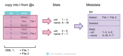
When inserting new entries into an existing table, it is essential to remember that files are unchangeable. This means that the new values cannot simply be added to the existing files. Instead, a new file must be created that contains the new values and expands the table in this way. Also, a new metadata snippet is added that records the added file and statistics about the data in this new file, such as minimal-maximal-value-ranges of each column.

If an entry in a table must be deleted, again, the file containing this entry cannot be changed directly. Alternatively, this file is replaced by a new one. To do this, all entries of the old file, except the one to be deleted, are copied to the new file. A new metadata snippet marks the old file as deleted, while the new one is added. Some statistics about the entries of the new file are also written to the metadata snippet.

With each new DML, a new metadata section is added, documenting which actions were performed by the DML and which new statistics apply. How this metadata management enables increased query performance will be explained in the following.

Select, Pruning, Time Travel and Cloning

Snowflake provides basic functionalities of query-based languages like select as well as special operations like time travel and zero-copy cloning. For all those operations, it uses metadata information to reduce the number of files to be queried. As a result, fewer files need to be loaded from cloud storage and scanned, which significantly improves query performance.

If a user queries a table so that the query could look like “SELECT * FROM table t”, the query optimizer first computes a scan set. This is the reduced set of files that is actually relevant for calculating the search result. Using the t table from the previous chapter, the scan set of the above query would include all files that are marked as added but not deleted in the metadata snippets, namely File 1, File 3, and File 4. Since the query does not contain a WHERE clause, there is nothing else to do except to send the scan set together with the query plan to the execution level to process it.

If a query has a pruning predicate, such as the query “SELECT * FROM table t WHERE user ID = 5”, the same scan set as described above is generated in the first step. The statistics of each file contained in the metadata snippets are then used to reduce the scan set further. As mentioned in the previous chapter, these statistics include the range of values for each column of a file. With this knowledge, Snowflake can easily compare the pruning predicate, user ID = 5, with these ranges. This way, it is possible to determine the file that actually contains the desired value; here, it is File 4. Now only this single file has to be processed in the execution layer, which is much faster than scanning all files of the original scan set.

Another function is time travel. Since the metadata sections can also contain timestamps, users can select files that existed at a specific time. This means that if a file is deleted at 3 pm and a user then asks for all the files that existed at 2 pm, he will also receive the deleted file. This is only possible because Snowflake never physically deletes a file, but only marks it as deleted. A corresponding query could look like “SELECT * FROM table t at (timestamp =>'2pm')”. In detail, the scan set is reduced to the state of the given timestamp before either an additional pruning predicate is executed or the query is sent to the execution level. For Snowflake users, this function is limited to 24 hours by default, allowing users to revoke any modifications made in this timeframe.

The zero-copy clone is a feature that extends the SQL standard to enable table cloning in a memory-saving and performant manner. Here, no real data is cloned in the cloud, only the metadata of the files. Hence the term zero-copy. An example would be the query “Create table t2 clone table t”. To perform such an operation, all metadata snippets of the source table t are combined in a new metadata snippet. This metadata is then assigned to the new table t2 and will be the basis for all future queries on this table. In combination with the time travel function, this technique allows the user to create a zero-copy clone of a table with its contents at a specific time. This can be useful for backup or testing purposes.

To improve the query runtime when pruning, Snowflake has implemented automatic clustering.

Automatic Clustering

While the first part of the talk explains how Snowflake stores data and manages metadata, the second part is about its automatic clustering approach.

Clustering is a vital function in Snowflake because pruning performance and impact depend on the organization of data.

Naturally, the data layout (“clustering”) follows the insertion order of the executed DML operations. This order allows excellent pruning performance when filtering by attributes like date or unique identifiers if they correlate to time. But if queries filter by other attributes, by which the table is not sorted, pruning performance is unfortunate. The system would have to read every file of the affected table, leading to poor query performance.

Therefore, Snowflake re-clusters these tables. The customer is asked to provide a key or an expression that they want to use to filter their data. If this is an attribute that does not follow the insertion order, Snowflake will re-organize the table in its backend based on the given key. This process can either be triggered manually or scheduled as a background service.

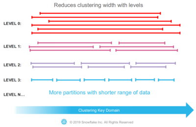
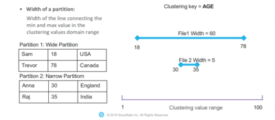
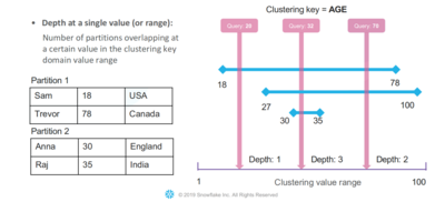
The overall goal of Snowflakes clustering is not to achieve a perfect order, but to create partitions that have small value ranges. Based on the resulting order of minimal-maximal-value-ranges, the approach aims to achieve high pruning performance.

This is illustrated using the example of a table perfectly ordered by an identifier column. Each partition has a range of ten values, while the total range goes from 1 to 100. If new data is added by the customer using DML operations with a range from 1 to 100, the newly inserted data affects every single file of that table. Every partition would have to be rebuild, leading to performance issues.

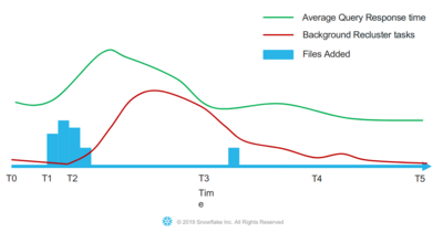
To keep up with DMLs, Snowflake has evaluated several approaches. One of them is re-clustering inline with the changes, meaning that all loads would be on the DML operations. Unfortunately, this increases the effort of DMLs, decreasing customer performance.

Another approach is batch re-clustering, in which a periodically triggered job would rebuild the table. This solution would be slightly better as DMLs are still fast, but the tables would be locked during the re-clustering process. For tables in Snowflake, which are up to petabyte sized, this would cost too much time to be applicable in practice. Also, the query performance degrades until then next clustering process starts.

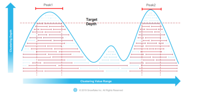
Hence, Snowflake decided to use incrementally re-clustering in a background task. Periodically, a small set of candidate files is re-organized to maintain an optimal performing table layout. This process repeats until query performance is at a satisfying level. Again, Snowflake does not aim for a perfect re-clustering but a balance between locking parts of the table and good clustering results.

To understand automatic incremental re-clustering, the basic functionality of Snowflake’s algorithm is explained. Data insertions trigger a process that uses metadata information to identify the files that need to be re-clustered to maintain query performance. In doing so, the system builds batches for re-clustering. Those will be re-sorted based on the correct clustering order given by the customer. Using an optimistic commit approach avoids locking the table during that process.

The crucial part of this algorithm is the partition selection. For this step, Snowflake is using metrics.

One of those is the “width” of a partition. The width is of the line connecting the minimal and maximal values in the clustering values domain range. Smaller widths are beneficial since they reduce the chance that a file is relevant for a high amount of queries.

That is why minimizing the partitions’ width leads to a higher pruning performance on average. The idea is to re-cluster the files that have the widest width, while this is inefficient when the data domain is very sparse.

The second metric that Snowflake primarily uses is “depth.” This metric is the number of partitions overlapping at a specific value in the clustering key domain value range. The use of depth is based on the insight that the performance decreases when a query scans several partitions. The more files are touched, the worse is the pruning efficiency.

To get consistency in that manner, Snowflake systematically reduces the worst clustering depth. All metadata is read, checking the value ranges. That way, depth peaks, in which the overlap is over a specified target level, can be identified. The partitions belonging to these peaks will be re-clustered.

However, it is essential not to re-organize small files, as they are the key to fast pruning. Modifying them could decrease performance in the worst case.

This fact is why Snowflake also takes clustering levels into account. The basic idea is to keep track of how often files have been re-clustered since this process leads to a width reduction on average. If a file has not been re-clustered yet, it is on level 0. Once re-clustered, it moves to the next level. Snowflake is using this system to ensure that files in clustering jobs have the same level. That way it provides, that already small files with excellent pruning performance do not increase their width in a cross-level re-clustering.

The part ends with an explanation of how automatic clustering affects query performance. When the customer inserts new data into Snowflake, the average query response time goes up. At the same time, the DML operations trigger background clustering jobs. Using the partition selection, Snowflake identifies the files that need to be re-clustered. After the re-clustering process, the query response time gets back down again.