Overview of the Lecture

In the lecture “Data Profiling: a Primer” Prof. Felix Naumann gives an engaging overview of current trends and topics in the field of data profiling. In particular, he first introduces the field and its applications and gives an overview of basic statistical approaches. Then, he presents his group's research results on three data profiling challenges: detecting unique column combinations, functional dependencies, and inclusion dependencies. Finally, he concludes with an outlook to further dependencies and other challenges.

Introduction to Data Profiling Tasks and Use Cases

Data profiling is the practice of reviewing and analyzing data to develop useful summaries. The procedure produces a high-level summary that users can use to identify data quality concerns, hazards, and general trends.

Data profiling use cases include query optimization, data cleansing, and data integration.

It can be used together with an ETL (extract, transform, load) procedure to cleanse, enhance, and load data into a destination location.

Profiling Tasks

Data profiling tasks appear at various granularities, especially in a database context. We can profile single columns to provide a better knowledge of the frequency distribution of various values, types, and uses for each column. Meanwhile, we can also profile the relation between multiple columns to discover properties, such as correlations between the columns. Finally, a dependency analysis can reveal hidden dependencies between different columns (not necessarily from the same table).

Single-column data profiling techniques include descriptive statistics, such as minimum, maximum, mean, or percentile. Further examples are calculating the standard deviation, frequency, variation, or aggregates, e.g., count and sum. Additionally, metadata, such as data type, length, uniqueness, or occurrence of null values can be of interest. We can use this metadata in turn to cleanse the data. For example, if we know that one column contains only unique values, we can easily filter out the faulty values that violate this uniqueness constraint. Further applications of this metadata are misspelling detection or finding missing values.

In the following, we are going to focus on three data profiling tasks for discovering data dependencies. The tasks include functional dependency discovery, uniqueness detection, and inclusion dependencies detection between different tables (indicating a foreign key relationship).

To make data profiling easier, purpose-built tools are usually utilized. When progressing from single column to single table to cross-table structural profiling, the computing complexity tends to increase. As a result, performance is a factor for evaluating profiling tools.

Data Profiling Use Cases

Data profiling use cases span a wide range of applications that we can perform once we have gained knowledge of the underlying data and profiled it.

One application is query optimization, where single-column profiling data, such as histograms and counts can help the optimizer of a DBMS to estimate cardinalities. As previously mentioned, data profiling can also be helpful for data cleansing. Here, the knowledge of data properties, such as the uniqueness of a column allows us to identify all violations of it. Furthermore, detecting dependencies across datasets is helpful for data integration tasks, e.g., finding foreign key relationships through inclusion dependency detection. Further use cases for data profiling are scientific data management, data analytics, and database reverse engineering.

Unique Column Combinations and Keys

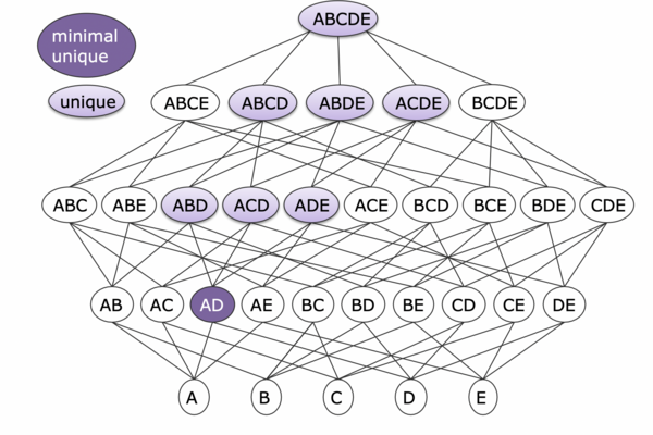
Unique column combinations (UCCs) extend the concept of unique columns. A column is unique if it has only unique values. Similarly, a column combination is unique if we have only unique value combinations from these columns. One can also say that the attributes of a UCC contain no duplicate entries in its projection.

Use cases

The knowledge of UCCs is crucial for defining key constraints for a relational dataset. For a set of columns to be a key, it is a necessary condition for them to be a UCC. However, only a domain expert can decide if a set of columns can be a key, because the possibility exists that the uniqueness of the values is just there by chance.

Typically, we are interested in finding minimal UCCs, where we can not remove a column without losing the uniqueness so we can find minimal keys. Additional use cases for UCCs include schema normalization, data cleansing, query optimization, and schema reverse engineering [4].

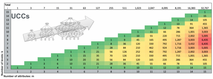
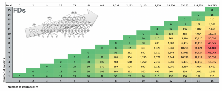
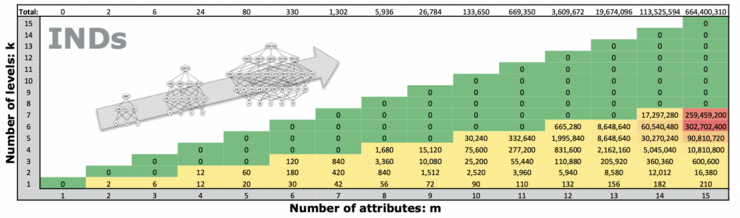
Problem Space

For a given table with m attributes, the number of possible UCCs of size k is m choose k. Thus, for m attributes, the overall number of UCC candidates to check is in O(2^m), which is exponential.

However, we can model this problem with a lattice structure. We can exploit the pruning properties of this structure to write efficient algorithms for finding UCCs. In the lattice, each UCC corresponds to one node.

Since we are only interested in key candidates, we are merely searching for minimal UCCs. In this example lattice, we found that the columns (A,D) are a minimal UCC. We know that all supersets of (A,D) are also unique. But we are not interested in these supersets since they can not be minimal. Thus, we can prune the entire search space above this minimal UCC.

Interestingly, we can even derive a similar pruning strategy when we traverse the lattice top-down. Then, all children of maximal non-unique column combinations are non-unique and we can prune them.

UCC Discovery Algorithms

There exist three classes of algorithms for discovering UCCs: column-based, row-based, and hybrid algorithms.

Column-based algorithms traverse the powerset lattice structure that we introduced above. The check if one node is a UCC is considerably expensive as it requires running through all of the data of the column combination. Therefore, depending on the traversal order (top-down, bottom-up, or hybrid), we can leverage pruning rules to reduce the search space.

DUCC, a column-based method, is an efficient UCC discovery technique currently available. This technique uses a random walk through the search space lattice to locate UCCs while maximizing the use of existing pruning criteria. This method is quicker than both GORDIAN and HCA [4].

In general, column-based algorithms grow well with higher numbers of records, but they become infeasible with large numbers of columns.

Meanwhile, row-based algorithms compare pairs of rows in a dataset. Per pair, they derive "agree or disagree sets," which are then used to generate UCCs [4]. This approach scales well with a high number of attributes but falls short for a large number of rows. An example of a row-based algorithm is GORDIAN [6].

Hybrid UCC discovery integrates approaches from column-based and row-based discovery algorithms into a single algorithm. Specifically, the HyUCC algorithm [4] automatically switches back and forth between the two methods. One challenge is to determine when to switch between the techniques. Furthermore, intermediate outcomes need to be converted from one model to the other model [4].

Functional Dependencies

Functional dependencies are constraints that specify the relation between two different sets of attributes. We write them in the form A → B, which means that given one value of column A, we know the value of column B for the same tuple.

Definition

Given two tuples t1, t2, if t1[A] = t2[A] then t1[B] = t2[B] must hold true. This implication also holds if we have sets of columns on the left or right side of the functional dependency. In the following, we abbreviate “functional dependency” with the term FD.

To make FDs tangible, the lecture gives the example of Game of Thrones characters. The FD 1. describes “if we know which person it is, we know their lineage”. This fact comes as no surprise, because we can think of the “Person” attribute as the key, which always has to determine all other columns.

FDs have several uses in database design. On the one hand, we can use FDs for the normalization of the schema design. By decomposing the tables into their normal forms (e.g., Boyce-Codd normal form, BCNF), we can eliminate functional dependencies between non-key attributes. These normal forms then help us to reduce duplication in the data, guarantee referential integrity, and protect from data anomalies.

In addition, we can leverage the knowledge of the FDs in data cleaning. Assuming we know that one FD is true for a database, we can find all violations of this FD and flag them as false values.

Further applications of FDs are query optimization and key discovery.

For all of the above applications, we require knowledge of the existing FDs in a database. FDs are another form of metadata that might often not be available. Therefore, we require algorithms to compute them.

Algorithm 1: Naive Approach to discover Functional Dependencies

The first algorithm that we consider is the naive approach of iterating through the entire search space.

for each column combination X

for each pair of tuples (t1, t2)

if t1[X\A] = t2[X\A] and t1[A] != t2[A]: break

With this, we want to find all functional dependencies X -> A for one column A. As there exist 2^(#attributes) different sets of column combinations, the complexity of this algorithm is O(2^#attributes * #rows^2), which is exponential.

Lattice Model and Column-Based Algorithms

We can model the problem with a lattice. Here, each edge represents one possible FD. For example, the edge AB -> ABC is equivalent to the FD AB -> C.

The problem space for finding FDs grows even faster than the one for Unique Column Combinations. The number of FDs to check in the lattice is equal to the sum of (m choose k) * (m - k) [1], which is exponential.

Similarly to the UCC lattice, different pruning rules apply:

• Given that we know a minimal FD A -> B exists (for the edge A -> AB, shown in purple in the lattice), the FD AB -> C is of no interest to us since it can not be a minimal FD. Therefore, we can prune the entire search space above the FD - edges we found.
• Likewise, we can prune from the top down. If we start at the top of the lattice and find a maximal non-FD, we are not interested in all edges below this FD since they can not be maximal. In the graph, this could be the FD CDE -> B. Therefore, we can prune all edges below this FD.

We can then use these pruning rules to write algorithms that visit only a much smaller number of edges.

Row-based FD Detection

An alternative algorithmic approach to finding FDs is the row-based approach. Here, we consider all possible pairs of rows of one table and use them to exclude FDs that can not be true based on the values of the rows.

For example, let us consider a table with two attributes “Name” and “Postcode”. We now check two rows t1 = (“Thomas”, “14482”), t2 = (“Sarah”, “14482”). Based on these rows, we know that the FD Postcode -> Name can not be true since we saw a counterexample.

With this approach, we can derive a set of knowledge about which FDs can not be true. Specialized algorithms are then able to derive the true FDs in the database. The complexity of this row-based approach is quadratic in the number of the rows, while the column-based approach rather scales with the number of columns.

Hybrid Algorithm HyFD

Hybrid algorithms, such as HyFD [2] combine the ideas of column-efficient and row-efficient FD algorithms. The main idea of HyFD is to go back and forth between the row-pair algorithm (Record Pair Sampler) and the lattice-based approach (FD Validator). The algorithm switches from the row-pair algorithm to the lattice once the information gain from new rows declines and goes back to the row-pair algorithm once it has gained new information on which rows to sample.

The performance of HyFD exceeded the performance of some of the previous algorithms by orders of magnitude. With this capability to detect hundreds of thousands of FDs for small datasets with only a double-digit number of columns, an entire new field of analyzing these FDs arises. In particular, one question is how we can distinguish between “spurious” FDs (that are just there by chance) and ground-truth FDs.

Inclusion Dependencies and Foreign Keys

Definition and Applications

Another kind of dependency that we want to detect is inclusion dependencies. An inclusion dependency R[X] <= S[Y] is defined for two tables R, S, and two sets of columns X and Y that have the same size. This inclusion dependency (IND) holds if the set of values of R[X] is a subset of the values of the other columns S[Y]. An inclusion dependency R[X] <= S[Y] is a necessary condition for X to be a foreign key in relation to Y. Thus, the prime use case for IND discovery is foreign-key detection. The foreign key discovery is a typical data profiling challenge as it helps us to determine which tables to join if we do not know the foreign key relationships. One example application is the work “Detecting Inclusion Dependencies on Very Many Tables” [3] that discovered INDs between millions of web tables and made them explorable with an interactive visualization.

Problem Space Dimensions

The problem space for IND discovery grows even faster than the one for FD discovery. For INDs, we have to consider all permutations of the columns. Therefore, the order of the columns matters. The number of INDs to check follows the sum over (m choose k) * (m-k choose k) * k!, which is exponential in m [1].

Interestingly, there are no candidates for k > m/2, because it only makes sense to have at maximum (m / 2) columns on one side of the IND and m / 2 columns on the other side.

References

This summary is based on the lecture “Data Profiling - a Primer” by Prof. Felix Naumann in the HPI Lecture Series on Database Research 2021/2022. All figures are taken from the lecture slides, if not specified otherwise.
[1] Papenbrock, T. (2017). Data profiling - efficient discovery of dependencies [Doctoral Thesis]. Universität Potsdam.
[2] Papenbrock, T., & Naumann, F. (2016). A Hybrid Approach to Functional Dependency Discovery. Proceedings of the 2016 International Conference on Management of Data.
[3] Tschirschnitz, F., Papenbrock, T., & Naumann, F. (2017). Detecting Inclusion Dependencies on Very Many Tables. ACM Trans. Database Syst., 42(3). doi.org/10.1145/3105959
[4] Papenbrock, T., & Naumann, F. (2017). A Hybrid Approach for Efficient Unique Column Combination Discovery. BTW 2017.
[5] Best practices to achieve optimal source data profiling. (2019, November 27). LightsOnData. https://www.lightsondata.com/source-data-profiling-best-practices/
[6] Sismanis, Y., Brown, P.G., Haas, P.J., & Reinwald, B. (2006). GORDIAN: efficient and scalable discovery of composite keys. VLDB.