Download
Introduction
When working with large amounts of automatically-crawled semantic data as presented in the Billion Triple Challenge (BTC), it is desirable to present the data in a manner best suited for end users. The Vocabulary of Interlinked Data (voiD) has been proposed as a means to annotate sets of RDF resources in order to facilitate human understanding.
In our paper Creating voiD Descriptions for Web-scale Data, we introduce automatic generation of voiD descriptions for automatically-crawled linked data. There, we describe different approaches for identifying (sub)datasets and annotating the derived datasets according to the voiD definition. Due to the complexity of the BTC dataset, the algorithms used for partitioning and augmenting the data are implemented in a Cloud environment utilizing the MapReduce paradigm. On this site, we present all these algorithms and visualize the derived results.
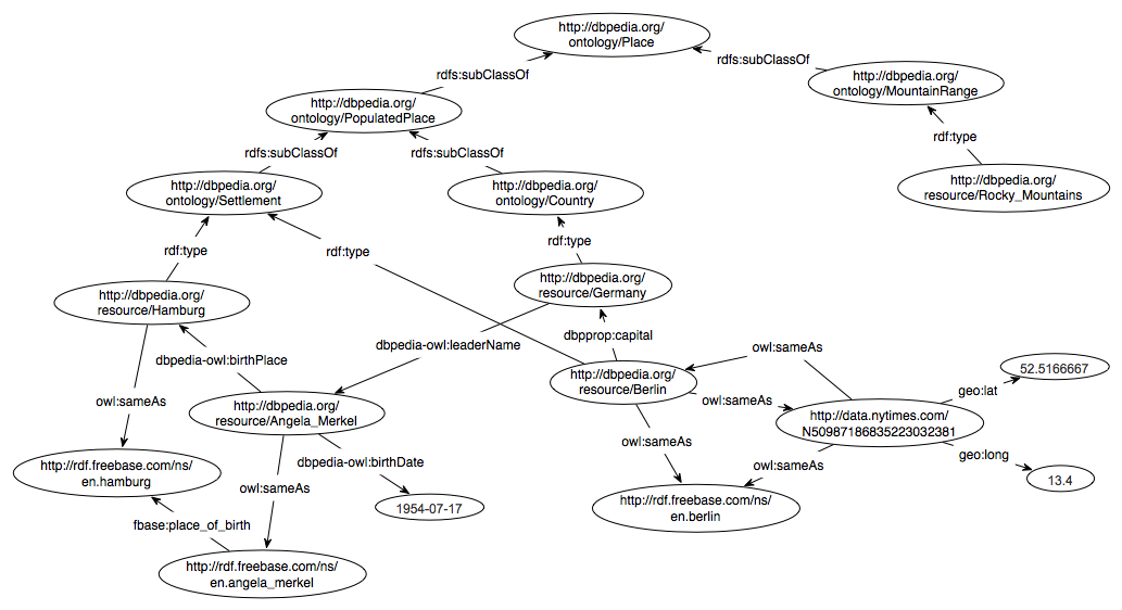
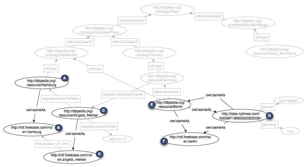
The results derived from applying our approaches to the dump of the Billion Triple Challenge 2010 are visualized in each subsection of this page; the raw output data can be downloaded there as well. To facilitate understanding, the following graph serves as a running example for some of the algorithms described:
RDF statistics
The RDF statistics provides some general information about the BTC dataset. We simply count the number of distinct subjects, predicates, objects and contexts. The number of difference resources altogether and the sum of all quadruples in the dataset are also determine.
Results
#subjects: 58,046,159
#predicates: 95,755
#objects: 94,524,583
#contexts: 8,097,413
#resources: 116,857,706
#quadruples: 3,171,184,130
Corrupted quadruples (e.g., containing literals with unescaped quote sign) are ignored.
URI-based clustering for void:Datasets
The URI-based clustering groups all entities that are provided by the same publisher into the same void:Dataset. As the publisher is identified by his or her void:uriLookupEndpoint, we determine the URL pattern of all subjects to categorize them. For instance, this approach identifies the dataset publishers dbpedia.org or rdf.freebase.com. This approach is described as the general case in the voiD guide.
Results (click for interactive SVG image)
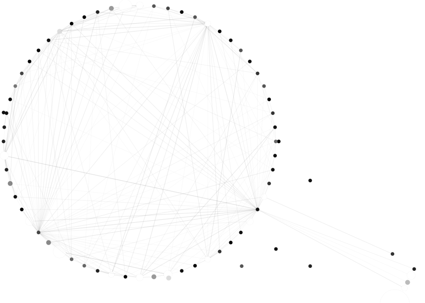
We reduced the number of displayed datasets in order to make the resulting graph more easily readable. In particular, we omitted all datasets that contain less than 100,000 entities. You can find the full results of our clustering algorithm below.
Results of the URI-based clustering
Connected clustering for void:Datasets
This approach enables dataset clustering in an adaptive manner. Nearly all information that is provided by an RDF triple/quadruple can be used for clustering the data in different ways. In our implementation all entities that are linked by a owl:sameAs predicate form one void:Dataset. This results in a number of datasets each consisting of several entities that might describe the same real-world object, but are provided by different publishers. This approach is a variant of the domain specific categorization suggested in the voiD guide.
Algorithm
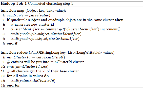
The data is processed using two separated MapReduce jobs. In the first job, a unique dataset id is attached to the subject and object of each RDF triple iff the associated predicate is equal to owl:sameAs. This is done during the Map step and outputs in a high number of datasets containing only two entities. Using this approach, an entity may end up in different datasets. Thus, we have to select one into which all associated datasets will be merged in. The Reduce step determines the minimal dataset id for each entity. All other dataset ids of this entity are now mapped onto this minimal dataset id as well.
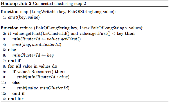
After processing the first job we have several datasets that contain entities and other dataset ids. These dataset ids reference other datasets that have to be merged into the current one. The second job generates the transitive closures of these void:subset in an iterative fashion. The job is executed several times until no more datasets can be merged into other datasets.
Sample
The following sample is based on the graph that was already shown in the introduction. The clustering in this example is based on the owl:sameAs predicate. All RDF entities that do not contain this predicate are omitted.
| | Input | Output |
| Map1 | A <owl:sameAs> B
C <owl:sameAs> D
E <owl:sameAs> F
E <owl:sameAs> G
G <owl:sameAs> E
G <owl:sameAs> F | A : 1
B : 1
C : 2
D : 2
E : 3
F : 3
E : 4
G : 4
G : 5
E : 5
G : 6
F : 6 |
| Reduce1 | A : [1]
B : [1]
C : [2]
D : [2]
E : [3, 4, 5]
F : [3, 6]
G : [4, 5, 6] | 1 : A
1 : B
2 : C
2 : D
3 : E
4 : 3
5 : 3
3 : F
6 : 3
4 : G
5 : 4
6 : 4 |
| Map2 (1) | Identify Mapper |
| Reduce2 (1) | 1 : [A, B]
2 : [C, D]
3 : [E, F]
4 : [3, G]
5 : [3, 4]
6 : [3, 4] | 1 : A
1 : B
2 : C
2 : D
3 : E
3 : F
3 : G
4 : 3 |
| Map2 (2) | Identify Mapper |
| Reduce2 (2) | 1 : [A, B]
2 : [C, D]
3 : [E, F, G]
4 : [3] | 1 : A
1 : B
2 : C
2 : D
3 : E
3 : F
3 : G |
Results (click for interactive SVG image)
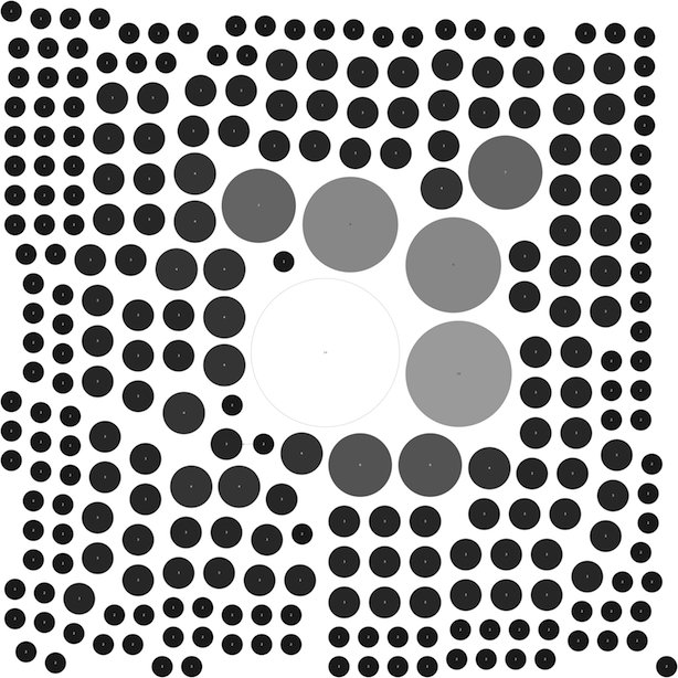
Results of the connected clustering
Hierarchical clustering for void:Datasets
This approach enables dataset clustering in a hierarchical manner. All entities that are instance of the same (upper) class form one void:Dataset. This results in a number of datasets each consisting several entities that might describe the same concept/class. We determine one void:Dataset for each hierarchy step, starting from the most specific class right up to the most general class. Therefore entities are part of one or more datasets.
Algorithm
The implementation of the hierarchical clustering is divded into three steps:
1. Optain list with explicit given subclass relations.
2. Iterative build-up of the transitive closure in k steps.
3. Joining instances to classes.
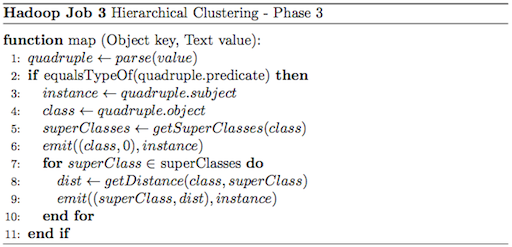
In the first step we identify all explictly given subclass relations and emit thise relations as SubclassHierarchyRecords. A SubclassHierarchyRecord represents a direct or undirected subclass relationship between two classes. We also store the distance d of the two classes along the hierarchy chain. By doining this, d = 1 for a direct subclass relation.
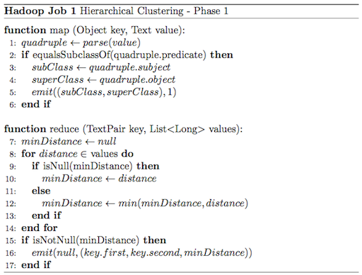
The second step contains the logic for the transitive closure. The first Mapper emits two outputs: (Subclass, SubclassHierarchyRecord) and (Superclass, SubclassHierarchyRecord). With it, potentially join partners (SubclassHierarchyRecords) will be grouped together in the Reducer. The Reducer joins the pairs and additional emitting all previous pairs. This MapReduce step is executed k times.
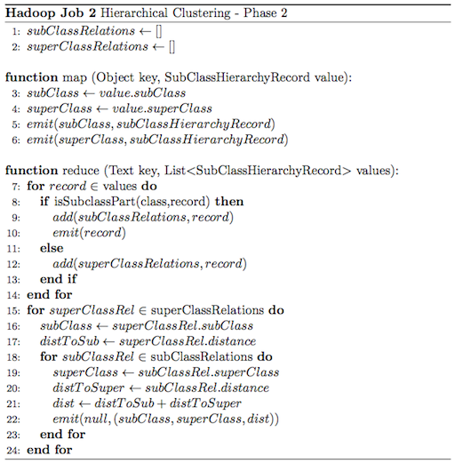
In the last MapReduce step instances and (upper) classes, with the corrsponding distance d, are joined together. After that, an identity reducer is executed.
Sample
The following sample is based on the graph that was already shown in the introduction. The clustering in this example is based on the rdf:type and rdfs:subClassOf predicates. All RDF entities that do not contain this predicate are omitted.

|
B <rdfs:subClassOf> C
C <rdfs:subClassOf> D
E <rdfs:subClassOf> D
G <rdfs:subClassOf> C | (B,C) : 1
(C,D) : 1
(E,D) : 1
(G,C) : 1 |
(B,C) : [1]
(C,D) : [1]
(E,D) : [1]
(G,C) : [1] | NULL : (B,C,1)
NULL : (C,D,1)
NULL : (E,D,1)
NULL : (G,C,1) |
NULL : (B,C,1)
NULL : (C,D,1)
NULL : (E,D,1)
NULL : (G,C,1) | B : (B,C,1)
C : (B,C,1)
C : (C,D,1)
D : (C,D,1)
E : (E,D,1)
D : (E,D,1)
G : (G,C,1)
C : (G,C,1) |
B : [(B,C,1)]
C : [(B,C,1), (C,D,1), (G,C,1)]
D : [(C,D,1), (E,D,1)]
E : [(E,D,1)]
G : [(G,C,1)] | NULL : (B,C,1)
NULL : (C,D,1)
NULL : (B,D,2)
NULL : (E,D,1)
NULL : (G,C,1)
NULL : (G,D,2) |
A <rdf:type> B
I <rdf:type> B
H <rdf:type> G
F <rdf:type> E
NULL : (B,C,1)
NULL : (C,D,1)
NULL : (B,D,2)
NULL : (E,D,1)
NULL : (G,C,1)
NULL : (G,D,2) | (B,0) : A
(B,0) : I
(G,0) : H
(E,0) : F
(C,1) : A
(D,1) : F
(C,1) : H
(C,1) : I
(D,2) : A
(D,2) : H
(D,2) : I
|
| Identify Reducer |
Results
Due to vast amount of certain predicate/object combinations (e.g., rdfs:subClassOf in combination with owl:Thing), our implementation incurred out of memory exceptions. Hence, we were not able to derive sensible results for hierarchical clustering within the entire BTC 2010 dataset. However, we evaluated our approach on a 10% sample.
Results of the hierarchical clustering (10% sample) - available upon request
Distinct clustering for void:Datasets
The distinct approach selects a single concept type per resource and assigns the resource to the respective dataset. The dataset selection is driven by the concepts' levels of generality. We use the concepts' occurrence rates to find out that level of generality, i.e., we consider frequent concepts to be more general whereas infrequent concepts have a lower level of generality.
Algorithm
This is a two-pass MapReduce job. Since one subject can be associated with multiple of rdf types the algorithm finds the best matching type for each subject in the input source. The best matching type for one subject is based on the number of subjects that the type describes in the whole dataset. Therefore, the first pass is used to build up statistical information about the types and the second pass will find the best matching type based on that information. The algorithm allows to change the strategy on which the best matching type is determined. In the following simplified example the best matching type is the most specific one, i.e. the type of the subject that describes the fewest other subjects as well. That strategy results in as many and as specific clusters as possible.
The first job's mapper takes each quadruple and emits two tuples with the object as the key if the predicate matches rdf#type. The first emitted tuple is used for counting the occurrences of that object as a type for a subject, therefore its value is just a 1. The second tuple is used for collecting all subjects associated with that type, that's why the value is the quadruple's subject.
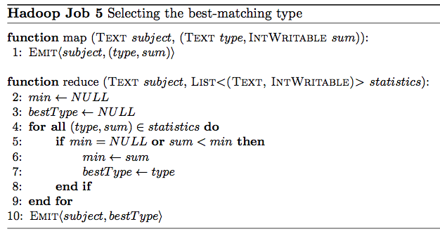
The first job's reducers now receive an object that is used as an rdf#type value as the key and a list of all subjects that are associated with that type as well as the number of occurrences that type is used in. The idea is now to emit each subject with the type as well as the number of overall occurrences of that type. In order to only buffer a small and constant amount of data we need to add up all occurrences before the first tuple needs to be emitted. To do that, we need to make sure that all tuples carrying occurrences arrive before all tuples carrying subjects. We do that by extending the output key of the first mapper with an index to be able to define the order of arrival at the reducers. Since the keys for one object are now different and would probably go to different reducers we needed to change the partitioning algorithm in a way that it ignores the index when hashing. That way all tuples with equal objects arrive at the same reducer even when the indexes differ. The sorting algorithm is untouched and takes both the subject and index into account, therefore tuples with the same subject but higher index will arrive after tuples with a lower index.
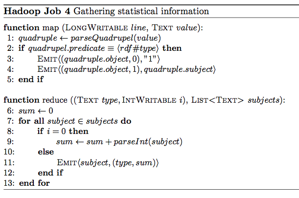
The second job's mapper is an identity mapper. The reducers work the following way: As long as the index of the compound (object,index)-key is zero, we interpret the value as an integer and add it up. When the index changes to one the values must be subjects and all occurrences must have been processed and stored in the sum variable. Then, for each subject we emit the subject and the type with its just computed overall usage count. The use of 1 as the value for occurrence tuples gives the opportunity to use a combiner in order to decrease network usage.
Sample
|
Berlin <rdf#type> City
Berlin <rdf#type> Capital
Potsdam <rdf#type> City | (City, 0) : 1
(City, 1) : Berlin
(Capital, 0) : 1
(Capital, 1) : Berlin
(City, 0) : 1
(City, 1) : Potsdam |
City : [1, 1, Berlin, Potsdam]
Capital : [1, Berlin] | Berlin : (City, 2)
Potsdam : (City, 2)
Berlin : (Capital, 1) |
| Identify Mapper |
Berlin : [(City, 2), (Capital, 1)]
Potsdam : [(City, 2)] | Berlin : Capital
Potsdam : City |
Results
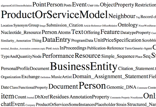
Larger font size indicates larger clusters.
 More results available upon request.
The Vocabulary of Interlinked Datasets specifies a number of properties that provide meta-information about each dataset to give an overview of its contents.
Algorithm
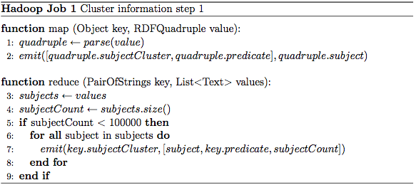
The dataset information is gathered using two different MapReduce jobs. The first task gathers statistical information about all predicates belonging to one dataset and counts the associated entities of each predicate. If predicates occur too often, they are omitted. The predicate information can used to identify the void:vocabulary of a dataset.
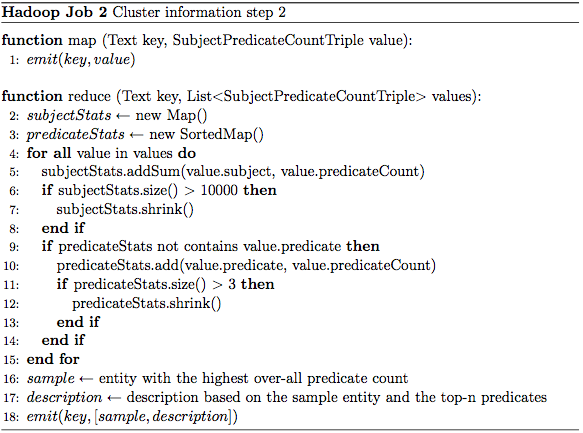
The second job analyzes the statistics and selects the entity with the most predicates as a void:exampleResource. Additionally we extract the three most common predicates as dcterms:description items in order to describe the dataset as advised by the voiD guide. Furthermore, we provide a rudimentary void:uriRegexPattern.
Results
The results of this algorithm are displayed in the tooltips of the connected clustering result graph.
Detecting void:Linksets
Linksets can be determined after applying any dataset clustering algorithm. A void:Linkset represents the connection between two different datasets and shows how strong these datasets are connected. The weight of one linkset is determined by the number of RDF triples that connects both datasets.
Algorithm
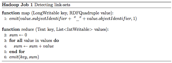
Detecting linksets is simple. Within the Map step all linksets are identified. We determine the subject's and the object's dataset ids and emit these values by concatenating them. The Reduce step simply counts the occurrence of each linkset. The final result contains all linksets and the number of their occurrences.
Sample
The sample is based on the graph that was already shown in the introduction and the connected clustering sample. We are now detecting all linkset, which means that all interlinked datasets are determined. Additionally, we assume for simplicity reasons in the sample below that all dataset identifiers are already available in the Map step (as mentioned above, dataset clustering is a prerequisite for linkset detection).
|
A <owl:sameAs> B
C <owl:sameAs> D
C <dbpedia-owl:birthPlace> A
C <dbpedia-owl:birthDate> "1964-07-17"
D <fbase:birthPlace> B
E <owl:sameAs> F
E <owl:sameAs> G
G <owl:sameAs> E
G <owl:sameAs> F
G <geo:lat> "52.5166667"
G <geo:long> "13.4"
... | 2_1 : 1
2_-1 : 1
2_1 : 1
3_-1 : 1
3_-1 : 1
... |
2_1 : [1, 1]
2_-1 : [1]
3_-1 : [1, 1]
... | 2_1 : 2
2_-1 : 1
3_-1 : 2
... |
Any links within the same dataset are ignored in the Map phase. If no dataset identifier can be determined (e.g., the entity is not contained in any dataset, or the object is a literal) the dataset id -1 is used. The sample run returns only one actual linkset: Dataset #2 and #1 are interlinked twice.
Results
The overall results are visualized in URI-based clustering and connected clustering result graphs by vertices between individual datasets.
Detecting used vocabularies
Each RDF triple uses a predicate to explain the semantics between its subject and its object. Therefore predicates are collected into RDFS vocabularies which describe how they are used correctly. The following algorithm tries to extract all used vocabularies.
Algorithm
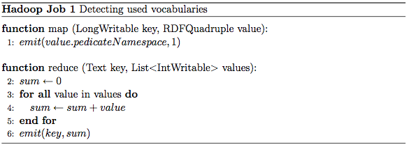
Detecting the vocabularies of a dataset can be done in the same way as described in the section above. We identify the vocabularies in the Map step and count their occurrences in the Reduce phase. The result contains all used vocabularies and the number of times each vocabulary occurred.
k-similarity
In addition to voiD linksets, we also examine links between different datasets that are not explicitly stated, i.e., 'fuzzy' linksets. We introduce the notion of k-similarity, where two subjects are k-similar, iff k of their predicate/object combinations are exact matches. The intuition is that two subjects are to some degree similar if they share a common set of attributes, and might therefore be relatable. This in turn helps to identify fuzzy linksets among datasets. These fuzzy linksets connect similar entities (and thereby datasets), which are not explicitly referenced by one another.
Algorithm
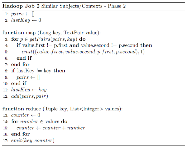
We employ two MapReduce runs for detecting fuzzy linksets. In the first one, all resources are clustered by their predicate/object combination. The Map step outputs hash values of these combinations as key, and associates the subject/context as value. The Reduce step is implemented as an IdentityReducer, i.e., the keys are only sorted for the second MapReduce job.

In the second MapReduce job, a Map-Side-Join is used to connect all similar subjects together. Here, all input values with identical key (predicate/object combination) are examined by the same map task of the second run. The map task discards all entries, where subjects and context are identical for the same key (i.e., two identical quadruples), while all other tuples of subject/context values with a common hash key are emitted. By counting them up in the Reducer step, we are able to identify the k-similarity of the two subject/context combinations.
Results
Due to vast amount of certain predicate/object combinations (e.g., rdf:type in combination with rdf:Resource), our implementation incurred out of memory exceptions. Hence, we were not able to derive sensible results for fuzzy linksets within the entire BTC 2010 dataset. However, we evaluated our approach on a 10% sample. Here, out of 317 million quadruples 122 million were at least 1-similar, but only 25 quadruples were at least 2-similar.

